Exploration
In this case I will be using simulation to explore a situation rather
than trying to
answer a particular question. I will be simulating the gender of the
driver in an
OPP random check of 100 vehicles (not including large truck etc. which
require
special driver's license) on the 401 for a given day of the year.
I aim to explore
how the composition of these samples can vary when the procedure is
repeated.
I will look at the proportion of male drivers in each sample and the
mean and
standard deviation of the data accumulated when the experiment is
repeated.
Plan
As an estimate of the probability of the driver of the car being male
or female
I used the data provided by the Ontario Ministry of Transport in its
2000
Ontario Road Safety Annual Report, Table 2.16 which provides Sex of
Driver
Population by Age Groups 2000. As part of the simulation I will assume
that
only Ontario drivers will be stopped.
Analysis
From Table 2.16 of the report 2000 Ontario Road Safety Annual Report
I find
that there are 4,313,694 male drivers out of a total of 8,121,374
licensed
Ontario drivers. Thus the probability that a random licensed Ontario
driver
is male is 0.531 (to three decimal places).
Since this is a two outcome experiment and if I assume that drivers
are
statistically independent the experiment suggests a Binomial Probability
model.
So, with a sample of 100 vehicles, the mean number of males driving
the cars
is given by
µ = np or µ = 53.1 males,
with a standard deviation of

However this does not provide me with an indication
of what could be the result in each sample. To get this view I tried
a simulation and to do this I followed the Instructions given in a
Fathom Workshop Guide (reference)

Procedures for the simulation of 100 Ontario
drivers.
| 1. I started with a new,
empty Fathom document |
|
| 2. From the shelf I dragged
a slider into the document |
 |
| 3. By double clicking
on the name V1 I changed it to probmale |
 |
| 4. I changed the slider
so that my scale would be approx 0 to 1 |
|
| 5. I set the slider to
the probability of randomly selecting a male drive, namely 0.531 |
|
| 6. I dragged a new
collection from the shelf |
 |
| 7. I double clicked on
the collection1 and renamed it Sample of drivers |
|
| 8. With the collection
selected I chose New Cases from the Data Menu |
|
| 9. I typed in 100 for
one hundred drivers in the dialogue box and clicked the OK |
|
10.
I double clicked on the collection which brought up its inspector
|
  |
| 11. In <new> I
typed driver and pressed Enter |
|
| 12. I double clicked
in the formula cell |
|
- 13. I typed in the following
- if(random()<probmale) and in the curly bracket
"male" in the top line and "female"
in the bottom line
|
 |
| 14. I closed the formula
editor by clicking the OK button |
|
| 15. I dragged a graph
from the shelf into the document |
|
| 16. Dragged the driver
attribute from the inspector onto the x axis.This gave me all that
I needed for the simulation. |
 |
| 17. To get a new set
of data from the simulation I chose Rerandomize from the
Analyze menu, and I explored the changes that occurred each
time I rerandomized. |
|
| 18. I looked at the effect
of changing the probability on the slider and then reset the probability
at 0.531 |
|
|

For further analysis I decided to accumulate
the data information of each 100 simulation and to see how these
data appeared graphically, what was their mean and standard deviation.
To do this I followed the instructions of the Fathom tutorial.
|
| 19.
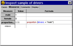
I opened the inspector window and clicked the Measures tab |
|
| 20. In <new>
I typed proportionOfMale for the measure's name |
|
| 21. I double clicked
in the formula cell |
|
|
22. I entered the formula
proportion(drivers="male")
|
  |
| 23. To ensure that
it was working I rerandomized a number of times and observed the
change in the proportionOfMale |
|
| 24. I closed the
Sample of Drivers inspector |
|
| 25. With the collection
selected, I choose Collect Measures from the Analyze
menu |
|
|
26. I double clicked the measures collection
to open its inspector
|
 |
| 27. Clicked on
the Collect Measures tab |
 |
| 28. Changed the
number of measures from 5 to 200 |
|
| 29. Finally clicked
Collect More Measures (this takes quite a while if the animation
is on) |
|
| 30. To look at
the results I brought a new graph onto the page |
|
| 31. I doubleclicked on
the sample of drivers collection to open its inspector |
|
| 32. Dragged the proportionOfMale
from the inspector to the x-axis of the graph |
|
| 33. Changed the graph
from a dot plot to a histogram |
 |
| 34. To get the mean and
standard deviation, I choose a Summary Table from the Insert menu |
|
| 35. Dragged the proportionOfMale
from the inspector to the top row of this table |
|
| 36. Noted the mean and
obtained the Standard Deviation by doubleclicking on S1=mean() and
changing it to stdDev(). |


|
REFERENCE:
Finzer, W. and Erickson, T., p. 25-27, "Tutorial 4: Simlation -
Polling Voters",
Workshop Guide for Fathom Dynamic Statistics(TM) Software Version
1.1, 2000. |
The results of the simulation follow:
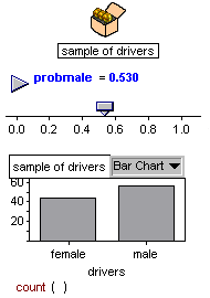
I introduced a slider for the probability of
stopping a male driver and set it to as
close to 0.531 as I could

Through the simulation I generated a table of the
sample data

from which I generated a Bar Chart of
the gender distribution for 100 drivers.
A typical distribution was

I then repeated the simulation 200 times,
in each case, noting the mean proportion of male drivers in each sample.
These 200 data were then plotted in a bar chart

and the mean and standard deviation
of this distribution was calculated


Observations
Through the simulation I saw that the sample composition of male and
female
drivers could change quite a bit from sample to sample, not only in
terms of totals
but also in the order in which they appeared. When this process was
repeated a
large number of times, the mean proportion of all the samples was
close to the
one on which I based my simulation, and although this number changed
slightly
as the number of repetitions was increased, it stayed consistently
close to 0.531,
which I noticed it is µ/n (where µ is the mean of the Binomial
distribution).
The
behaviour of the standard deviation was a bit more erratic than that
of the mean
but it did move around the value of 0.05. I explored to see whether
this was
related to any of the values that I used in the simulation. I found
that it is close to
the sqrt(.431x.469) and is therefore also close to ó/sqrt(n) (where
ó is the
standard deviation of the Binomial distribution).
>>NEXT