Fechner's Law and the Method of Equal-Appearing Intervals
Louis L. Thurstone
University of Chicago
The purpose of the present experiment was partly to ascertain whether Fechner's law holds for a certain kind of stimulus but primarily to bring out certain limitations of the method of equal-appearing intervals and the ways in which some of them may be overcome.
One of the best known examples of the method of equal-appearing intervals in the experimental verification of Fechner's law is the Sanford weight experiment.[1] The envelopes are so weighted that they present as far as possible the same appearance and that they are in all respects identical except as to their weights. The subject is asked to sort out these envelopes into five piles so that the piles seem to be equally spaced as to apparent weight. Each pile of envelopes is weighed and then it is easy to ascertain the average weight of the envelopes in each of the five piles. The five equally-spaced S-values, the five successive piles, are then plotted against the average weight of the envelopes in each of the five piles. The plot is expected to be logarithmic to satisfy Fechner's law. This procedure involves a methodological error which can be avoided by the procedure to be explained.
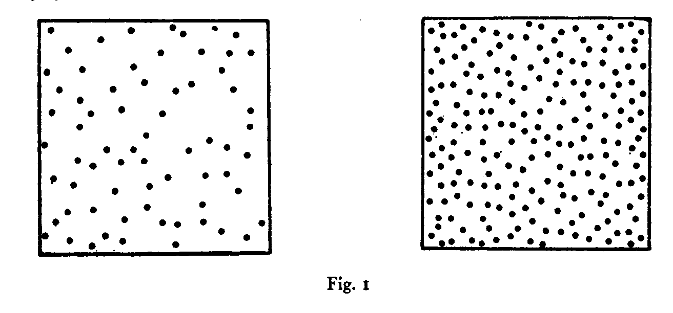
The stimuli for the present experiment consisted of a series of 96 cards. On each card was printed a 2 1/2-inch square which was filled with irregularly spaced dots. The stimulus magnitude was the number of dots in the square. The lowest and the highest magnitudes are illustrated in Fig. 1. They were arranged in a geometrical series of 24 steps from 68 dots to 198 dots. Each stimulus magnitude was represented by four cards in the series. The subject was given
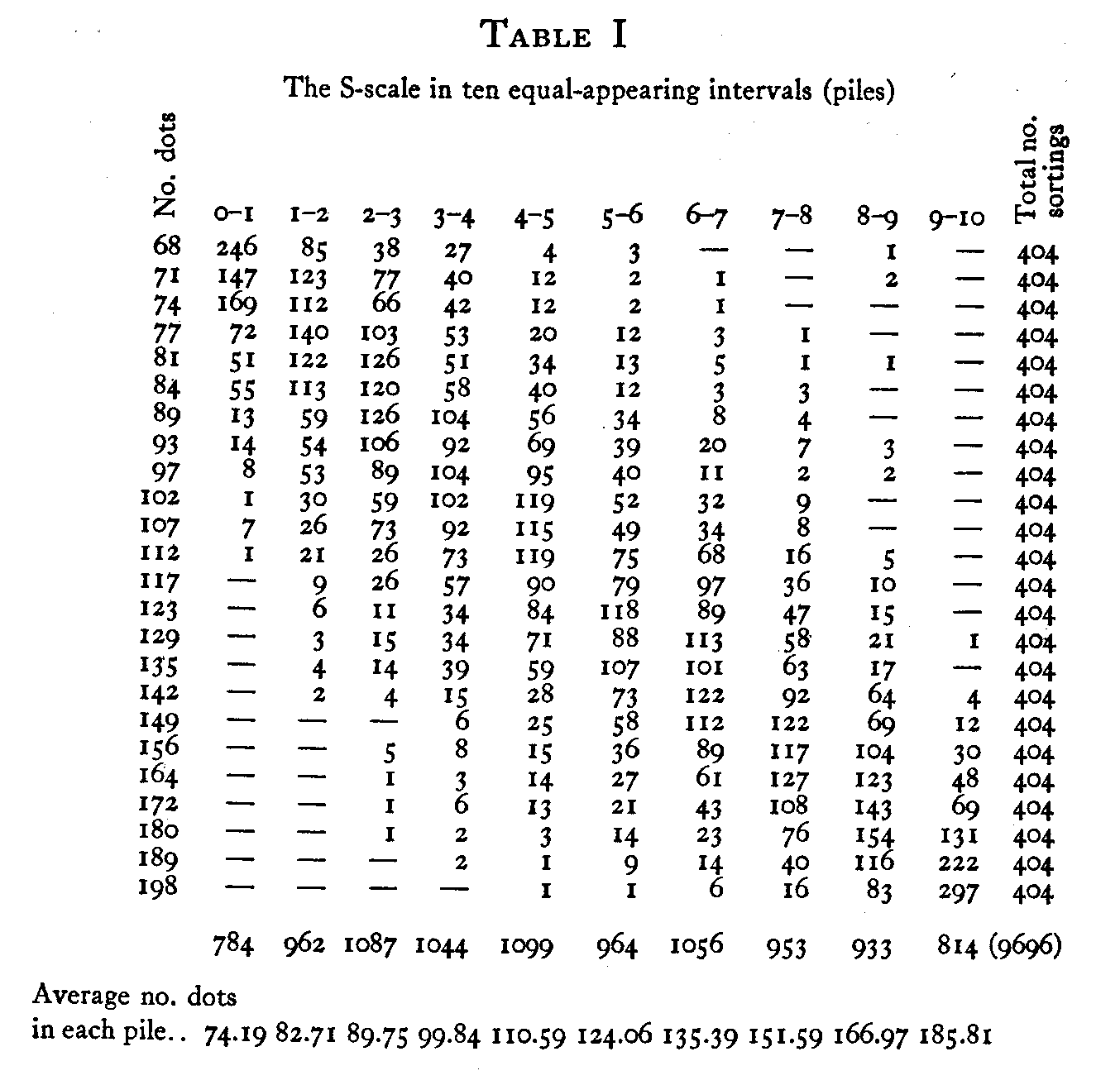
( 215) the pile of 96 cards and asked to sort them out into ten piles which should constitute as far as possible a series evenly graduated as to the apparent density of the dots on the cards. There were l01 subjects in the experiment so that there were 404 sortings for each stimulus magnitude.
The raw data are summarized in Table I. The S-scale is represented by ten equal class intervals, the ten piles. The R-scale is represented by the number of dots on the card.
Fechner's law is a statement of the relation between these two variables. It is usually written in the form
S = K log (R), (1)
in which S is the allocation of the stimulus to the psychological or discriminal continuum, and R is the stimulus magnitude, the number of dots. In order to provide for any units of measurement for R and S, and in order to provide for an arbitrary origin on the S-scale it is desirable to write the equation in the more flexible form
S = K log (CR). (2)
This equation is easily rectified by writing it in the form
S = K log R + K log C, (3)
in which K log C is a constant. The verification of Fechner's law would be complete if the plot of S against log R should be linear. If this plot is not linear, then Fechner's law is not verified. This assumes, of course, as in any experimentation
( 216)
of this type, that there is sufficient curvature to the plot S against R so that its rectification by the above logarithmic plot is convincing.
The detailed interpretation of the table is as follows. There were 246 sortings in which cards containing 68 dots were placed in the first or lowest of the ten piles. The cards containing 68 dots were placed in the second of the ten piles 85 times. It is to be expected that the cards with relatively low stimulus magnitudes (number of dots) should be placed in the lowest piles while the cards with the large number of dots should be placed in the higher numbered piles. This is seen to be the case in that there is a drift of entries in the table from the upper left-hand corner to the lower right-hand corner. Since each stimulus magnitude was sorted 404
( 217) times, the sum of the entries in each row is 404. The piles were designated as equal class intervals on the S-scale and the origin for the scale is placed arbitrarily at the lower edge of the lowest of these ten class intervals. For this reason the entries in the first of the ten columns can be handled as class frequencies for the interval 0 � 1 on the S-scale. The next column represents the frequency of sortings of each stimulus magnitude for the class interval 1 � 2 and so on.
In order to ascertain whether Fechner's law holds, it is necessary to compare the S- and R-values, which are expected to give a logarithmic plot. In the present instance there can hardly be any ambiguity about the stimulus magnitude which is simply the number of dots in the square. We must decide, however, on a method for determining the S-value which is to be assigned to each stimulus magnitude. At this point appears the methodological error which is involved in the well-known Sanford weight experiment, which has been quoted by Titchener and others. If we should proceed as in the Sanford weight experiment, we should merely ascertain the average number of dots in each pile. These would be considered as the adjusted R-values to be plotted against the equal intervals on the S-scale. As a matter of fact such a procedure makes use of the wrong regression for this problem.
In many experimental problems it is necessary to ascertain which of two regressions is to be used. Whenever the object is prediction one should use the regression "unknown on known." In the present case we are not interested in predicting S-values from known R-values, or vice versa. We are interested in the intrinsic relation between S and R. In such a situation one should minimize experimental discrepancies in the variable which is least accurately measured. In this case there can be no doubt that the S-value is far more inaccurate than the R-value, which is merely the number of dots on the card. Consequently we should adjust the S-values against constant R-values. The regression "Son R" assumes that the R-values contain no error and that is for all practical purposes true. Probably the only error in the present R-values is the very slight fluctuation in the diameters
( 218) of the dots by which apparent density might conceivably be affected. But this error is almost infinitesimal compared with the discrepancies in the S-values, the apparent magnitude. In a situation in which both variables are measured with equal accuracy, and in which no problem of prediction is involved, one should fit the data by a function intermediate between the two regressions. For linear functions this is easily done, but non-linear functions for such experiments are sometimes troublesome.
The instructions for the Sanford weight experiment call for the regression R on S, which is a violation of good experimental practice. We shall use the correct regression in this case which is S on R. This necessitates that we ascertain an S-value for each of the 24 stimulus magnitudes. Inspection of our table shows immediately that the distributions represented by the horizontal rows are by no means normal. They are banked toward the end piles by the "end-effect." Merely to ascertain the arithmetic mean of the piles is there-fore not a suitable procedure. This objection also holds against the incorrect procedure of the Sanford weight experiment in which the student is asked merely to ascertain the
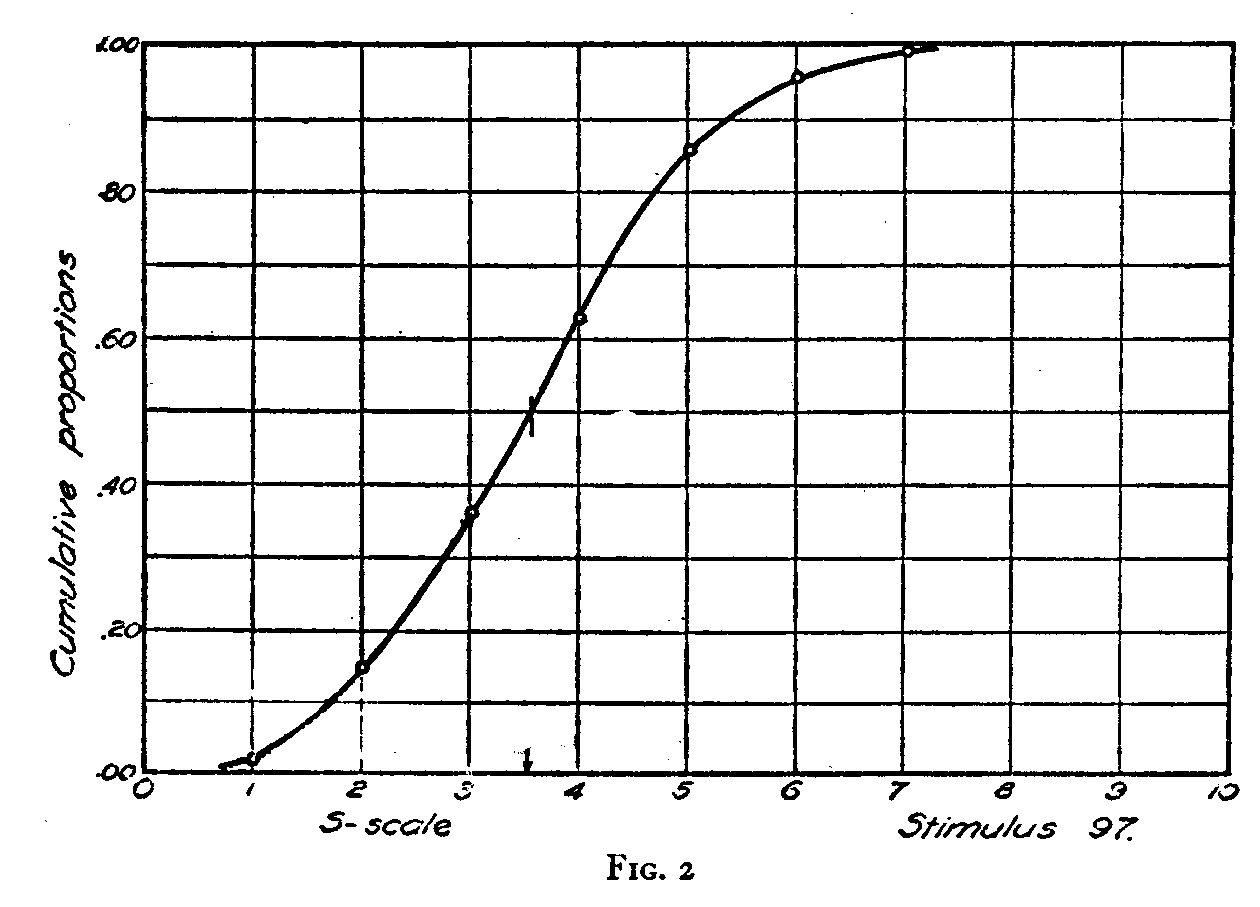
( 219) average weight per envelope in each pile. We have adopted the median S-value for each stimulus magnitude as the most suitable measure of central tendency on the S-scale. For this purpose a cumulative frequency distribution was drawn for each of the horizontal rows of the table. An example of this procedure is illustrated in Fig. 2 for stimulus magnitude 97. The class frequencies for the R-value of 97 have here been represented in a cumulative frequency distribution of the percentile form. The median S-value is the S-value at which the smoothed curve reaches an elevation of .50, which is 3.55 for the stimulus 97. This means merely that half of the subjects perceive this stimulus as larger than 3.55 on the S-scale, while half of them perceive it as smaller than that apparent magnitude. One cumulative frequency diagram was drawn for each stimulus so that there were 24 diagrams for this experiment similar to Fig. 2.
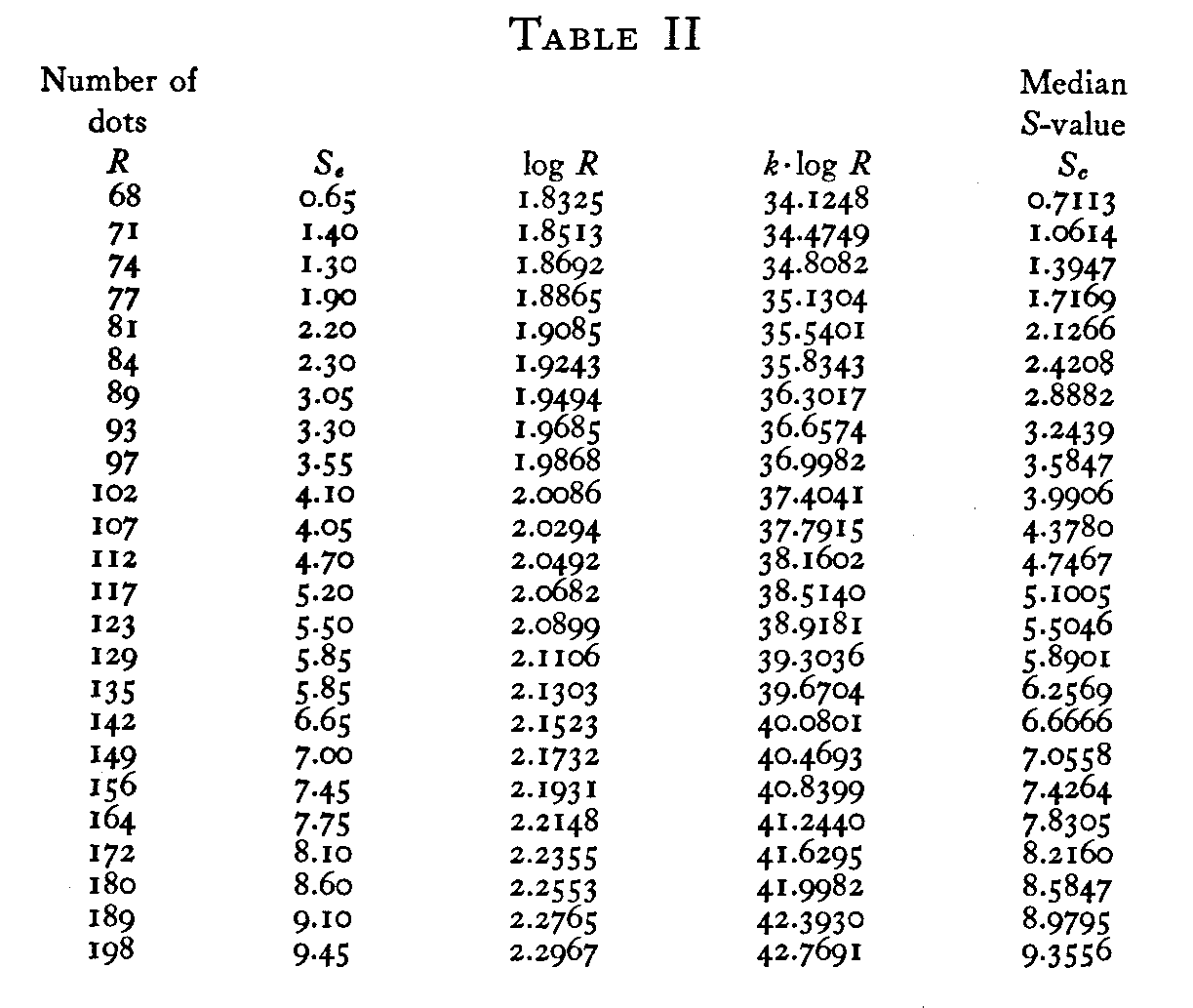
We now have the experimental S-values, Sc. They are listed in Table 2. We are now ready to determine whether
( 220)
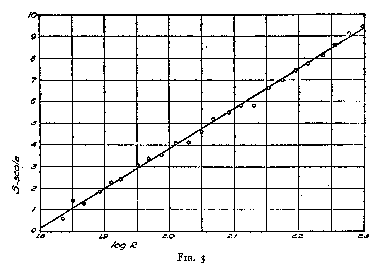
the linearity of Equation 3 is satisfied by the experimental data. The values of log R are also listed in the same table. In Fig. 3 we have plotted S against log R as indicated by Equation 3. The linearity of Fig. 3 is immediately apparent.
Its slope is the constant K in Equation 3, and the S-intercept is the constant K log C. These constants may be determined by the method of least squares; but for the present problem that may hardly be necessary. The linearity of Fig. 3 constitutes final proof that Fechner's law holds for the stimuli of the present experiment. If Fig. 3 had been non-linear, it would have disproved Fechner's law for the present experiment. The straight line of this figure was drawn by inspection so that approximately as many points may be found on one side of the line as on the other. The constant K is determined graphically to be 18.621 and the S-intercept is also determined graphically to be — 33.4135.These two values would undoubtedly shift slightly by different methods of fitting the line of Fig. 3 such as the method of least squares, the method of averages, or Reed's method of minimizing normals.[2] But for our purposes such slight fluctuations in the constants are not of importance.
( 221)
The column K log R of Table II can then be filled in since the constant K has been determined. The last column of this table shows the calculated S-values, Sc. These are obtained again from Equation 3 with the known values for K, K log C, and the known stimulus magnitudes.
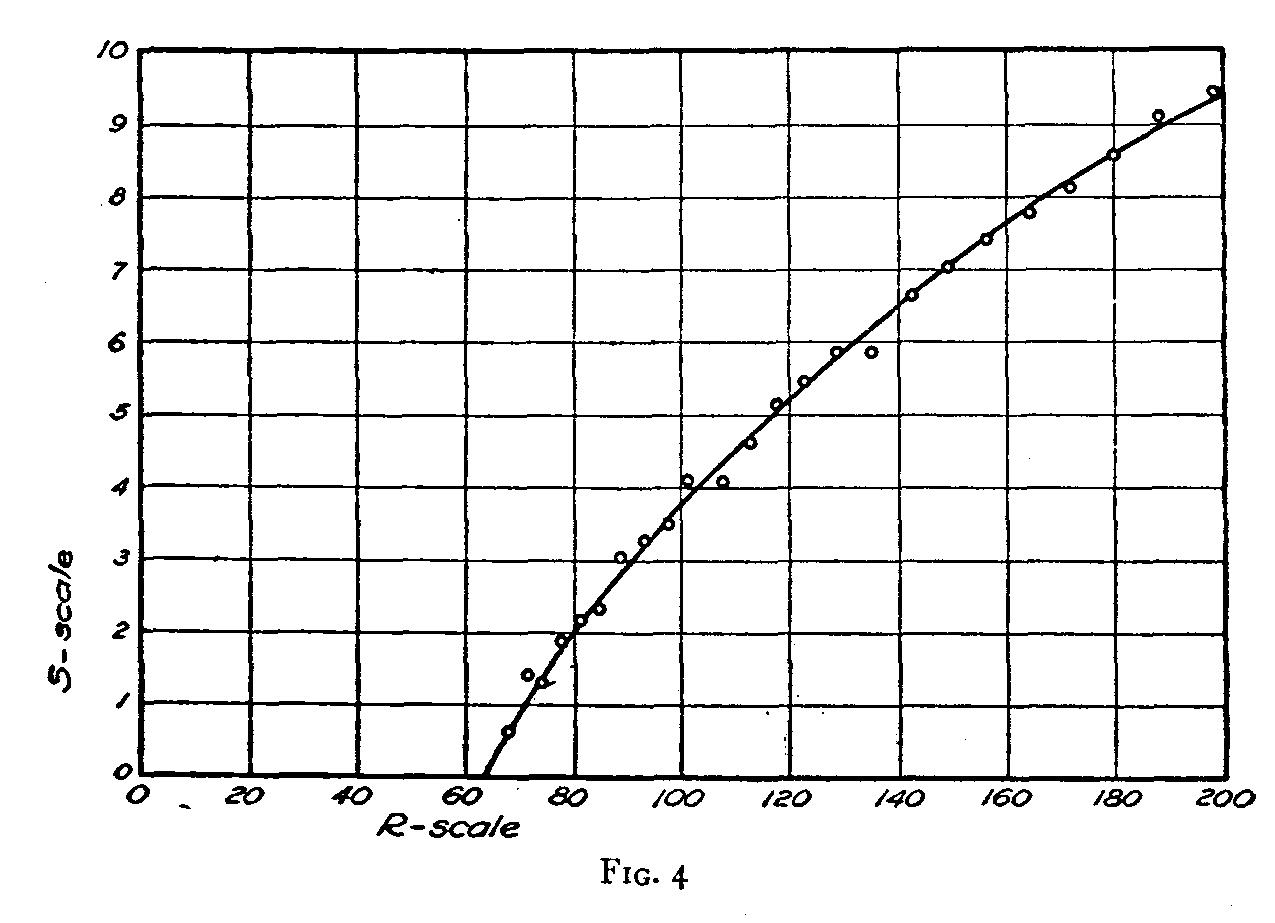
In order to ascertain the magnitude of the experimental discrepancies from Fechner's law we have drawn Fig. 4. The small circles represent the experimental S-values, Sc, which have been plotted against the corresponding stimulus magnitudes. These data are obtained directly from Table II. The smooth curve has been drawn through the calculated S-values, Sc, of this table. This diagram shows rather clearly that experimental deviations from Fechner's law are very slight in the present experiment and we are therefore justified in concluding that the law has been verified.
There are several psychological and methodological considerations that are fairly well illustrated in this simple experiment. The final equation of the curve of Fig. 4 is
S = 18.621 log R — 33.4135.(4)
One might inquire about the psychological meaning of this
( 222) equation when S is zero. In that case R takes the value 6z. In other words, when there are about 62 dots on the card the S-value according to our equation should be zero. This is entirely sensible because the origin for the S-scale is arbitrary. In fact, according to Fechner's law, in its most general form, Equation 1 automatically prescribes an origin for the S-scale for unit stimulus magnitude. In the present case, 62 dots on the card happens to be unit stimulus magnitude for the law in its simplest form. There is no psychological ambiguity about this fact if we remember that we are dealing with an arbitrary origin on the S-scale. Naive interpretation might ask whether the apparent magnitude is zero for unit stimulus magnitude. But such a question is of course entirely irrelevant when S-measurements are made from an origin arbitrarily assigned to unit stimulus magnitude.
The same question may appear in slightly different form by inquiring about negative values for S. Myers[3] speaks of a "difficulty" about Fechner's law in that it leads to negative sensations. Any value for anything can be negative if you place the arbitrary origin high enough. And so in this case the S-value for a stimulus would be negative if the unit stimulus magnitude is arbitrarily assigned high enough. Consequently negative S-values in Fechner's equation do not mean that the apparent magnitude is less than nothing. This alleged difficulty with Fechner's law is caused by failure to understand the meaning of Fechner's simple equation. The issue simply does not exist.
It is of some interest to study the dispersion that a stimulus projects on the S-scale. This can be done by inspecting the data of Table I. The inspection shows the end effect rather conspicuously. This effect can probably be explained most simply in terms of the mechanical restrictions of the method of equal-appearing intervals. The subject adopts a scale of subjective magnitudes for the ten piles and when he sees an unusually large stimulus magnitude he may have the impulse to place it in pile 12 or pile 15 if such piles were available or allowable. Since he is restricted to ten
( 223) piles, he sorts all of these large apparent magnitudes in pile 10. Undoubtedly the next stimulus which is slightly smaller is affected by such a restriction so that it is sorted into piles 8 or 9 instead of into 10 or 11. The same effect is seen at the lower end of the S-scale. For this reason we cannot deal with the distributions of Fig. 4 as in any sense true projections of the stimuli on the S-scale. They are subject to gross distortions by the mechanical limitations of the method of equal-appearing intervals. It is of course possible that we are also dealing with an adaptation effect caused by familiarity with the experimental stimulus range, and that this may itself constitute a source of distortion in addition to the mechanical limitation of the method of equal-appearing intervals. It is probably not so great as that of the restraint to a specified number of piles. There would seem to be good reason to assume that the distribution of the stimulus magnitude 198 should be approximately the same in form as the distribution for the stimulus magnitude 68. Consequently if we want to study the dispersion that a stimulus projects on the S-scale we must resort to other psychophysical methods than that of the method of equal-appearing intervals. In fact this is one of the most serious limitations of that method. It is entirely absent in the method of paired comparison, which is probably the best of all the psychophysical methods.
Another serious limitation of the method of equal-appearing intervals for which I can offer no solution is that the determinations are undoubtedly affected by the distribution of stimulus values which the experimenter happens to use. In the present case we use 24 stimulus magnitudes in a geometric series from 68 to 198 dots. If we had so selected the same number of stimuli as to constitute an arithmetical series with the same range, the subject would have been compelled to make the tenth pile rather large while the first pile would be rather small. It is almost certain that the subject would have been confused by the fact that his sortings gave gradually increasing piles from the first to the tenth. He might unwittingly disturb his scale of apparently equal intervals in an attempt to make the class frequencies in the
ten piles roughly equal. On the other hand, the same question may be raised as a criticism against our procedure, in which the stimulus magnitudes constituted a geometric series. If the subject sorts the stimuli into ten successive piles with instructions to make all of the ten piles approximately equal in size and without any instructions to make the intervals between them equal, then we should automatically verify Fechner's law, provided we were to interpret the intervals to be equal even though the subject were never told to make them so. This is a serious limitation in the method of equal-appearing intervals by which our confidence in this psycho-physical method should be markedly disturbed. Whenever it is at all possible we certainly should avoid the method of equal-appearing intervals and use instead the method of paired comparison or one of its equivalents.
(Manuscript received August 21, 1928)